Data Science · Case study · 2024
Learning rewards from behavior
An academic project, implemented from scratch. Instead of learning how to act given a reward, Inverse Reinforcement Learning asks the opposite question: given how an agent does act, what reward was it pursuing? This write-up rebuilds the full Bayesian IRL pipeline — environment, forward solver, demonstrations, and the PolicyWalk sampler — and reports honestly what the experiments show.
01
The problem: inverting RL
Classic reinforcement learning takes a reward function and searches for a policy that maximizes it. Inverse reinforcement learning (IRL) flips the arrow: we observe an agent behaving — a sequence of states and the actions it chose — and we try to recover the reward function that best explains that behavior.
This matters whenever the reward is the hard part. Hand-specifying what we want an agent to value is notoriously brittle; it is often easier to demonstrate good behavior than to write down its objective. IRL is the formal route from demonstrations back to objectives.
The Bayesian framing, following Ramachandran & Amir (2007), treats the reward function as a random variable: we place a prior over reward functions, define a likelihood of the observed actions given a reward, and sample from the resulting posterior. The goal of this project was to build that entire chain by hand, in a controlled gridworld, to understand each moving part.
02
The environment: a gridworld MDP
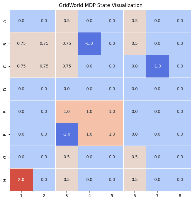
Everything happens on an N×N grid modeled as a Markov Decision Process. Each cell is a state; the actions are the four moves L, R, U, D. The world is stochastic: with probability 0.8 a move goes where intended, and with a slip probability of 0.2 the agent veers to a perpendicular cell instead. The discount factor is γ = 0.9. Moves that would leave the grid keep the agent in place.
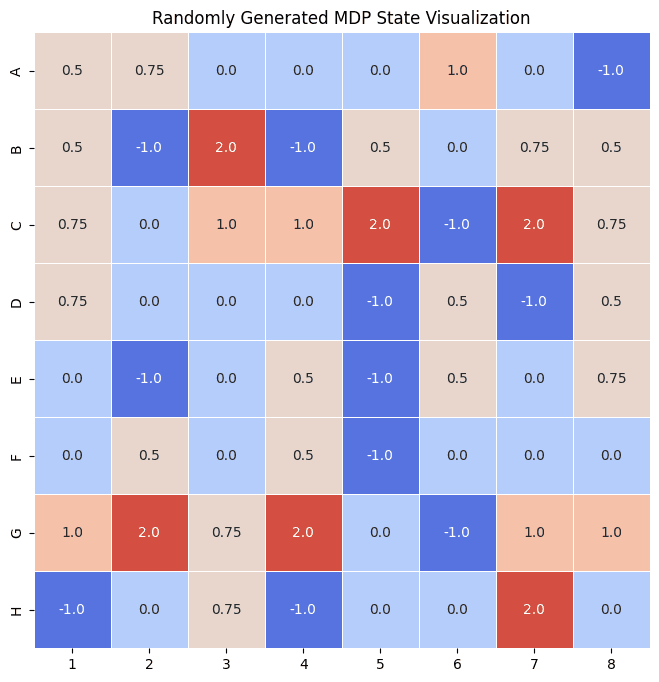
To stress-test the method beyond one hand-crafted map, a second class RandomPartialMDP populates the grid with random semantic features — Treasure, Bomb, Mud, Water, Mountain — each mapped to a reward value. This gives an endless supply of fresh worlds to evaluate the algorithm on.
03
Solving the forward problem: Policy Iteration
Before we can invert anything, we need to be able to solve the forward problem — given a reward, find the optimal policy. I implemented Policy Iteration with the three classic steps:
- Evaluation — iteratively compute the value of every state under the current policy until it converges.
- Improvement — at each state, switch to the action with the best expected value.
- Iteration — repeat evaluation and improvement until the policy stops changing.
This solver is the workhorse reused throughout the rest of the project: every candidate reward proposed by the Bayesian search is turned into a policy through Policy Iteration.
04
Generating demonstrations: an imperfect tutor
IRL needs observed behavior to learn from. Rather than assume a perfect demonstrator, I built an imperfect tutor: it mostly follows the optimal policy, but with a 5% chance picks a random action (optimal_action_prob = 0.95). Starting from an initial state, it rolls out a trajectory and records the resulting sequence of (state, action) pairs.
This noise is deliberate and realistic — real demonstrators make mistakes — and it is exactly what the Bayesian likelihood is designed to tolerate, rather than requiring the observations to be perfectly consistent with a single reward.
05
The Bayesian framework
With an environment, a solver, and demonstrations in hand, the inference machinery has three pieces.
Priors over rewards
I implemented three candidate priors — UniformPrior (any reward within a bound is equally likely), GaussianPrior (rewards near zero are favored, penalizing extreme values), and BetaPrior. The Gaussian prior is the one carried through the experiments.
Likelihood: a Boltzmann policy
The likelihood links a reward to the observed actions. For a given reward we compute the Q-values (via a value-iteration-style sweep), then assume the tutor picks actions with a softmax / Boltzmann distribution over those Q-values: P(a | s) = exp(α·Q(s,a)) / Σ exp(α·Q(s,·)). The parameter α encodes how rational (deterministic) the agent is assumed to be. The likelihood of a set of observations is the product over all observed (state, action) pairs.
Posterior and acceptance ratio
The posterior is simply prior × likelihood. Because we will compare candidate rewards rather than normalize, the key quantity is the ratio of posteriors P(R₁ | O) / P(R₂ | O) — exactly what a Metropolis-Hastings sampler needs to decide whether to accept a new proposal.
06
PolicyWalk: sampling the reward space
PolicyWalk is the MCMC algorithm at the heart of Bayesian IRL. The reward space is too large to explore exhaustively, so we random-walk through it: start from a random reward, repeatedly propose a small perturbation to a neighboring reward, recompute the induced policy, and accept the proposal with probability min(1, posterior(R')/posterior(R)). Over many steps this traces out the posterior — concentrating on rewards that explain the demonstrations well.
The recovered reward vectors are directly interpretable: a positive value marks a state the agent is inferred to find desirable, a negative one a state it avoids. Reading them back against the grid is the qualitative sanity check that the inference is doing something sensible.
A simulated-annealing variant
I also implemented CoolingPolicyWalk, which adds simulated annealing: a temperature T that decays each iteration and reshapes the acceptance probability via exp(Δlog-posterior / T). Early on, high temperature permits exploratory, occasionally-worse moves; as T cools, the walk settles toward high-posterior regions. The aim is to escape poor local optima that a plain walk can get stuck in.
07
Evaluation: 0-1 policy loss
How do we score a recovered reward? Not by comparing reward numbers directly — many different rewards induce the same optimal behavior — but by behavior. The 0-1 policy loss is the fraction of observed (state, action) pairs where the policy implied by the recovered reward disagrees with what the tutor actually did. I compared plain PolicyWalk against the cooling variant across grid sizes 5, 8, and 10.
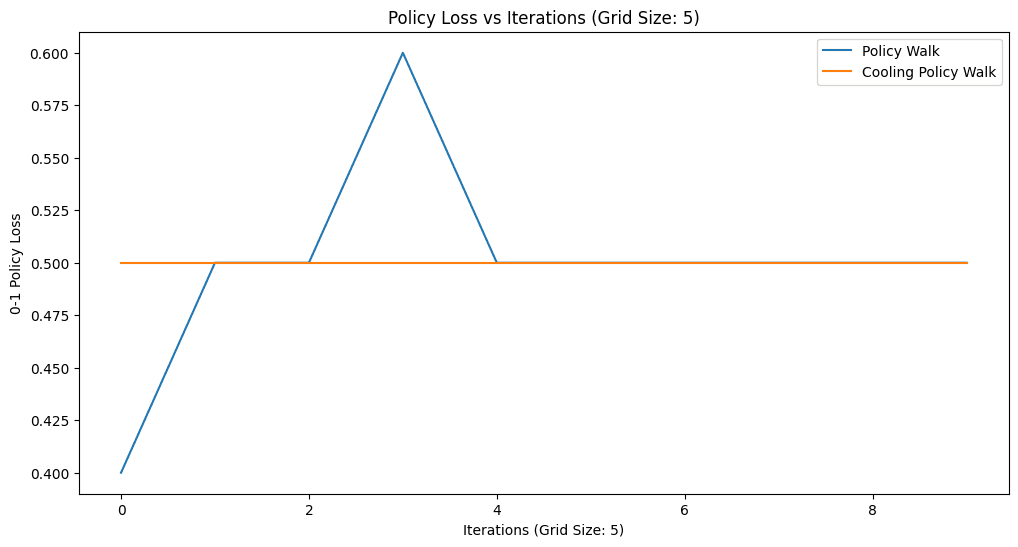
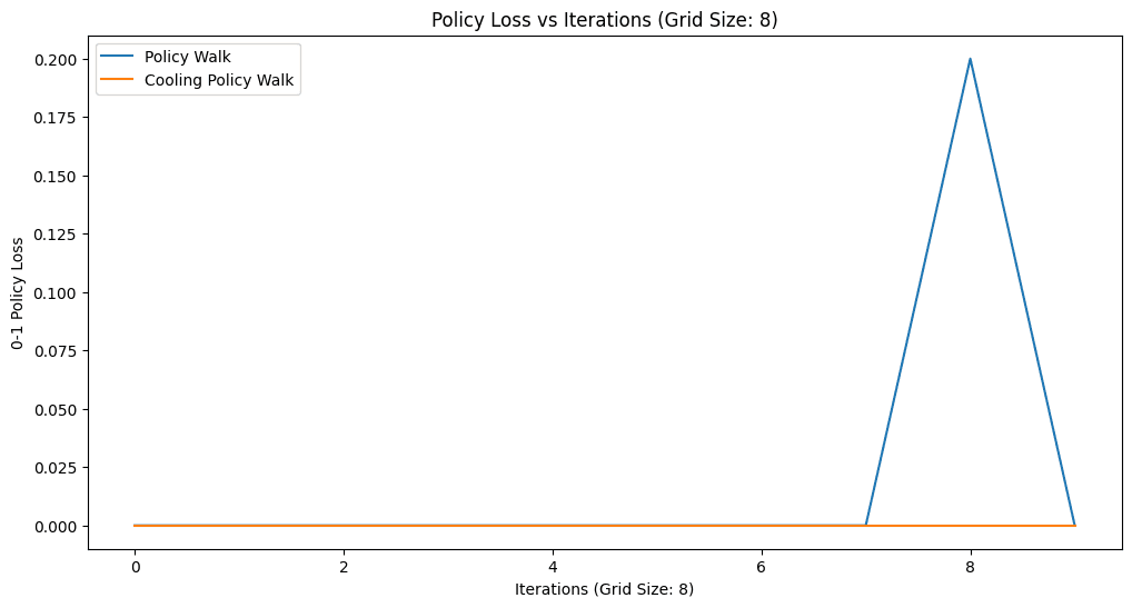
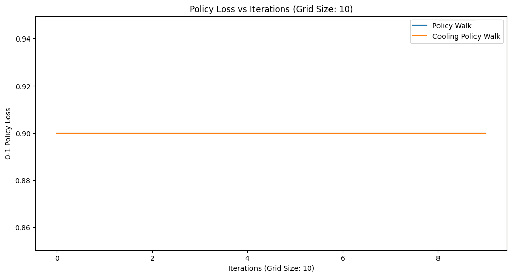
The honest reading: the results are mixed and noisy, and that is itself informative. PolicyWalk is high-variance — it can find a zero-loss reward (grid 8) but does not reliably stay there. The cooling variant trades that volatility for stability, but on these runs stability sometimes means being stuck. On the 10×10 grid both struggle, illustrating how the reward posterior gets harder to explore as the state space grows and the demonstrations stay short.
08
Takeaways
This was a from-scratch build rather than a polished product, and the value is in what it forced me to understand end to end:
| Component | What it demonstrates |
|---|---|
| MDP + stochastic transitions | Modeling sequential decisions under uncertainty |
| Policy Iteration | Dynamic programming, the RL forward problem |
| Imperfect tutor | Realistic, noisy demonstrations |
| Priors, Boltzmann likelihood, posterior | Bayesian modeling from first principles |
| PolicyWalk (MCMC) | Metropolis-Hastings sampling over a structured space |
| Simulated annealing variant | Exploration vs exploitation in samplers |
| 0-1 policy loss across grid sizes | Behavior-based evaluation, honest reporting |
What I take away: implementing a method from the paper up — environment, solver, likelihood, sampler, evaluation — teaches far more than calling a library. The noisy results aren't a failure to hide; they show the real difficulty of reward inference, and reading them honestly is part of the work.